Evaluation of Bioinformatics Methods
Cross-Validation Technique
Cross-validation is a statistical method for validating a predictive model. Subsets of the data are held out, to be used as validating sets, a model is fit to the remaining data (a training set) and used to predict for the validation set. Averaging the quality of the predictions across the validation sets yields an overall measure of prediction accuracy.
In cross-validation, the original data set is partitioned into smaller data sets. The analysis is performed on a single subset, with the results validated against the remaining subsets.
The subset used for the analysis is called the “training” set and the other subsets are called “validation” sets (or “testing” sets).

Jack Knife Test
Jackknifing, which is similar to bootstrapping, is used in statistical inferencing to estimate the bias and standard error in a statistic, when a random sample of observations is used to calculate it. The basic idea behind the jackknife estimator lies in systematically recomputing the statistic estimate leaving out one observation at a time from the sample set. From this new set of "observations" for the statistic an estimate for the bias can be calculated and an estimate for the variance of the statistic.
K-fold Cross-validation- For each of K experiments, use K-1 folds for training and a different fold for Testing .This procedure is illustrated in the following figure for K=4

· Advantage of K-Fold Cross validation is that all the examples in the dataset are eventually used for both training and testing.
· Disadvantage of this method is that the training has to be completed k times, meaning it takes k times as much computation time
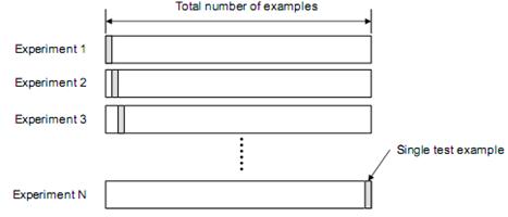
Leave-one Out Cross-validation- Leave-one-out is the degenerate case of K-Fold Cross Validation, where K is chosen as the total number of examples.
· For a dataset with N examples, perform N experiments
· For each experiment use N-1 examples for training and the remaining example for testing.
Advantage: Makes best use of the data
Involves no random sub sampling
Disadvantage: Very computationally expensive and stratification is not possible.
Bootstrapping Technique
Bootstrapping technique is a statistical method for estimating the sampling distribution of an estimator by sampling with replacement from the original sample, most often with the purpose of deriving robust estimates of standard errors and confidence intervals of a population parameter like a mean, median, proportion, odds ratio, correlation coefficient or regression coefficient. It is often used as a robust alternative to inference based on parametric assumptions when those assumptions are in doubt, or where parametric inference is impossible or requires very complicated formulas for the calculation of standard errors.
Sample a dataset of n instances n times with replacement to form a new dataset of n instances. Use this data as the training set. The remaining examples that were not selected for training are used for testing .Randomly select (with replacement) N examples and use this set for training. The remaining examples that were not selected for training is used for testing .This value are likely to change from fold to fold.
Repeat this process for a specified number of folds (K).

Monte Carlo Method
Monte Carlo methods are a class of computational algorithms that rely on repeated random sampling to compute their results. This method often used when simulating physical and mathematical systems. This can be loosely described as a statistical method used in simulation (a method that utilizes sequences of random numbers as data) of data.
Monte Carlo methods are used to solve various problems by generating suitable random numbers and observing that fraction of the numbers obeying some property or properties. The method is useful for obtaining numerical solutions to problems which are too complicated to solve analytically.
As this method is mainly depend upon random number. So, random number is unique every time. For example a dataset of 200 sequences generate random number (24, 19, 74, 38, 45, 38, 45, 38, 45, 38, 45) .Here the number 38 and 45 repeat many times. This will unnecessarily waste time and give bias model that is not accurate.
Advantage: As number of iteration is better will be the result. For example 10000 iterations give more accurate result as compared to 100 iterations.
Disadvantage: Like any other statistical methods any bias in random number generator will affect the results.
If the model develop during training is wrong, the result may be wrong.
 |
|||
|
|||
NOTE: The tie between the bootstrap and Monte Carlo simulation of a statistic is obvious: Both are based on repetitive sampling and then direct
examination of the results. A big difference between the methods, however, is that bootstrapping uses the original, initial sample as the population
from which to resample, whereas Monte Carlo simulation is based on setting up a data generation process (with known values of the parameters).
Where Monte Carlo is used to test drive estimators, bootstrap methods can be used to estimate the variability of a statistic and the shape of its
sampling distribution.
Three Way Split Technique
If model selection and true error estimates are to be computed simultaneously, the data needs to be divided into three disjoint sets.
Training set: A set of examples used for learning: to fit the parameters of the classifier.
Validation set: A set of examples used to tune the parameters of a classifier.
Test set: A set of examples used only to assess the performance of a fully-trained classifier.
Flow Chart shows the Stepwise procedure of three way split technique
PROCEDURE OUTLINE:
1. Divide the available data into training, validation and test set
2. Select architecture and training parameters
3. Train the model using the training set
4. Evaluate the model using the validation set
5. Repeat steps 2 through 4 using different architectures and training parameters
6. Select the best model and train it using data from the training and validation sets
7. Assess this final model using the test set
Dis-Joint Test
Two sets are said to be disjoint if they have no element in common. eg- A={1, 2, 3} and B={4, 5, 6} are disjoint sets. This definition can be extends to any collection of sets. A collection of sets is pairwise disjoint or mutually disjoint. eg- Set A={1, 2}, Set B = {2, 3} and Set C= {3, 1} the intersection of the collection A, B and C is empty, so this is mutually disjoint set but the collection is not pairwise disjoint. In fact, there are no two disjoint sets in the collection.
Criteria using disjoint sets
Number of element/sequences in each set is at least 30.
Set must be pairwise disjoint set otherwise there is bias during training that will result in over prediction.
It is important that the test set is not used in any way to create the classifier.
Procedure Outline:
1. Make Positive and Negative datasets in two files. eg- N number sequences for positive and N number for negative sequences.
2. Combine these two file in two a single file.eg- N+N=2N
3. Make X no. of sets that are pair wise disjoint set means not two sets have common element/sequence and also not a single element/sequence is repeated in a single set.
4. Make Training set and Test set like
5. Training Set Test Set
I) Set-1+Set-2+Set-3+Set-4 Set-5
II) Set-1+Set-2+Set-3+Set-5 Set-4
III) Set-1+Set-2+Set-4+Set-5 Set-3
IV) Set-1+Set-3+Set-4+Set-5 Set-2
V) Set-2+Set-3+Set-4+Set-5 Set-1
6. Now Run SVM Learn on each Training Set and SVM Classifier using corresponding Test Set.
7. Select the best model that shows accurate results.
Non-redundant Five-fold Cross-validation
Ideally sequence in dataset should have minimum sequence similarity (e.g., less than 30% in case of proteins) but it decrease size of dataset significantly. The performance of SVM model directly proportional to size of dataset used for training. We can use non-redundant five-fold cross validation technique, where sequences in dataset were clustered based on sequence similarity. These clustered were divided into five sets; it means all sequences of a cluster were kept in one set. Thus no two sets have similar sequences; it means sequences in training and testing sets have no sequence similarity. We can make clusters using Blastclust and CD-HIT even blastall may also use for this purpose. By using this technique we make non-redundant dataset without decreasing dataset size.
Measuring Performance
 |
|
Predicted
|
Actual |
|||
|
|
Positive |
Negative |
|
|
|
Positive |
TP |
FP |
PPV |
|
|
Negative |
FN |
TN |
NPV |
|
|
|
Sensitivity |
Specificity |
|
|

Figure: Criteria of classification of a prediction into TP, TN, FP and FN
Threshold Dependent Parameters
Example: 203 people were examined for checking the probability of lung cancer
|
Predicted |
Actual |
|||
|
|
Positive(sick) |
Negative (Healthy) |
|
|
|
Positive (Sick) |
TP=2 |
FP=18 |
PPV =2 / (2 + 18) =10% |
|
|
Negative (Healthy) |
FN=1 |
TN=182 |
NPV =182 / (1 + 182) =99.5% |
|
|
|
Sensitivity =2/(2+1) =66.67% |
Specificity =182/18+182 =91% |
|
|
· True positive (TP) : Sick people correctly diagnosed as sick
· False positive (FP) : Healthy people wrongly identified as sick
· True negative (TN) : Healthy people correctly identified as healthy
· False negative (FN) : Sick people wrongly identified as healthy
Sensitivity or percentage coverage of positive is the percentage of positive example predicted as positive.

A sensitivity of 100% means that the test recognizes all sick people as such. Thus in a high sensitivity test, a negative result is used to rule out the disease.
Sensitivity alone does not tell us how well the test predicts other classes (that is, about the negative cases). In the binary classification, as illustrated above, this is the corresponding specificity test, or equivalently, the sensitivity for the other classes.
Specificity or percentage coverage of negative is the percentage of negative examples predicted as negative.

A specificity of 100% means that the test recognizes all healthy people as healthy. Thus a
positive result in a high specificity test is used to confirm the disease. The maximum is trivially achieved by a test that claims everybody healthy regardless of the true condition. Therefore, the specificity alone does not tell us how well the test recognizes positive cases. We also need to know the senstivity of the test to the class, or equivalently, the specificities to the other classes.
Probability of Positive Correct Prediction (PPV)
The positive predictive value is the proportion of patients with positive test results who are correctly diagnosed.

Probability of Negative Correct Prediction (NPV)
The negative predictive value is the proportion of patients with negative test results who are correctly diagnose.

Accuracy is the degree percentage of correctly predicted examples (both correct positive and correct negative prediction).

= (2+182/2+182+18+1) × 100 = 90.64%
Matthews Correlation Coefficient is used in machine learning as a measure of the quality of binary (two class) classifications. It takes into account true and false positives and negatives and is generally regarded as a balanced measure which can be used even if the classes are of very different sizes.
It returns a value between -1 and +1. A coefficient of +1 represents a perfect prediction, 0 an average random prediction and -1 an inverse prediction.
The
Matthews Correlation Coefficient is generally regarded as being one of the best
such measures. ![]() In
this equation,
In
this equation,
= (2×182) - (18×1)/sqrt ((2+18) × (2+1) × (118+18) × (118+1)
= 346/sqrt (971040)
= 0.371
If any of the four sums in the denominator is zero, the denominator can be arbitrarily set to one; this results in a Matthews Correlation Coefficient of zero, which can be shown to be the correct limiting value.
Threshold Independent Parameter
Receiver operating characteristic (ROC) or simply ROC curve is a graphical plot of the sensitivity vs. (1- specificity) for a binary classifier system as its discrimination threshold is varied. The ROC can also be represented equivalently by plotting the fraction of true positives (TPR = true positive rate) vs. the fraction of false positives (FPR = false positive rate) also known as a Relative Operating Characteristic curve, because it is a comparison of two operating characteristics (TPR & FPR) as the criterion changes.
ROC analysis provides tools to select possibly optimal models and to discard suboptimal ones independently from (and prior to specifying) the cost context or the class distribution. ROC analysis is related in a direct and natural way to cost/benefit analysis of diagnostic decision making. ROC analysis has more recently been used in medicine, radiology, psychology, and other areas for many decades, and it has been introduced relatively recently in other areas like machine learning and data mining.
AUC: The area under the ROC curve, is called Area under the curve (AUC), or A' (pronounced "a-prime"). If AUC value is more than 0.5 then our model is working well otherwise it’s a worse model.

Reliability Index
Reliability index is a simple indication of level of certainty in the prediction. This RI calculated by the following given equation-
![]()
RI is used in multiclass classification study. Assignment of RI to each sequence based upon the difference of highest and second highest score of various 1-vs-rest SVMs in multi-class classification.
Regression Method
Regression/Real Value: We used machine learning techniques in regression/real-value prediction. In this we predict real value as melting point, boiling point, IC50, Kd, EC50 etc. These are the parameter which gives explanation how good predicted values are good in compare to its real value. To access model performance and provide statistically meaningful data, we can calculate different statistical parameters. Here I am giving formulas using melting point (MP) as an example.
|
Actual MP |
Predicted MP |
|
12.5 |
14.0 |
|
67.0 |
71.3 |
|
71.2 |
68.7 |
|
115.9 |
121.0 |
|
32.7 |
29.8 |
|
45.7 |
49.3 |
|
79.8 |
76.8 |
|
127.3 |
125.1 |
|
57.6 |
50.2 |
|
37.2 |
33.8 |
|
|
|
|
|
|
![]() = 53297.66
= 53297.66
Mean
(![]() ): The arithmetic mean is the
"standard" average, often simply called the "mean".
): The arithmetic mean is the
"standard" average, often simply called the "mean".
![]()
So here mean of actual ![]() =
12.5+67.0+71.2+115.9+32.7+45.7+79.8+127.3+57.6+37.2/10
=
12.5+67.0+71.2+115.9+32.7+45.7+79.8+127.3+57.6+37.2/10
= 646.90/10 = 64.69
Similarly ![]() =
14.0+71.3+68.7+……../10
=
14.0+71.3+68.7+……../10
= 640.00/10 = 64.0
Pearson's correlation/Sample correlation (R): In general statistical usage, correlation refers to the departure of two random variables from independence. R is the Pearson's correlation coefficient of actual and predicted value, this give idea about the performance of machine learning techniques.

R = 53297.66 – 646.90*646.0/sqrt (53580.21 - 646.902)*(53169.64 – 646.002)
= 11896.06/11968.56
= 0.994
Where n is the size of test set, MPpred is the predicted melting point and MPact is the actual melting points. Value of R always ranges from -1 to +1 negative. Negative value of R shows that there is inverse relationship within actual and predicted value; while positive value of R show that here positive relationship within actual and predicted value. If R = 0 then it’s totally random prediction.
Coefficient of determination (R2): Coefficient of determination is the statistical parameter for proportion of variability in model.

Sum of square of errors (SSE) = ![]()
Sum of square of total (SST) = ![]()
Where MPpred is the
predicted melting point and MPact is the actual melting points![]() is the mean
of MPact.
is the mean
of MPact.
R2 = 1 – (SSE/SST)
=1 – (154.53/11732.249) = 0.87
The coefficient of determination is also the arithmetic average of all M folds run. Value of R2 always ranges within 0 to 1. Its value gives idea how these actual values are related with predicted value. Higher values of R2 show that here linear relationship within actual and predicted and lower value shows that non-linear relationship
Q2 is another very important statistical parameter for the determination of variability in model.

![]()
If value is more 0.5 then models performance is good.
RMSE is the root mean squared error of the predictions calculated according

= sqrt (154.53/10)
= 3.931
Where n is the size of test set, MPact is the actual melting point and MPpred is the predicted melting point by different machine learning techniques. Like mean absolute error it’s also give idea how our predicted melting point is for away from actual melting points.
MAE/AAE is mean of absolute errors within actual and predicted value
![]()
= 1/10* (| 12.5-14.0| + |67.0-71.3|+ …..)
= 3.59
Its gives idea how our predicted value are for away from experimentally calculated melting point. Where n is the size of test set, MPact is the actual melting point and MPpred is the predicted melting point by different machine learning techniques.
RMSECV is the aggregate root mean squared error of the cross-validation. For an M fold cross-validation, it is defined as

Statistical Method
z-Test- The Z-test compares sample and population means to determine if there is a significant difference.
It requires a simple random sample from a population with a Normal distribution and where the mean is known.
Calculation The z measure is calculated as:
Z =
(x - m) / SE
where x is the mean sample to be standardized
m is the populations mean, SE is the standard error of the mean.
SE = s / sqrt(n)
where s is the population standard deviation, n is the sample size
The z value is then looked up in a z-table. A negative z value means it is below the population mean (the sign is ignored in the lookup table).
· The Z-test is typically with standardized tests, checking whether the scores from a particular sample are within or outside the standard test performance.
· The z value indicates the number of standard deviation units of the sample from the population mean.
Note: z-test is not the same as the z-score, although they are closely related.
t-Test- The t-test assesses whether the means of two groups are statistically different from each other. This analysis is appropriate whenever you want to compare the means of two groups.
![]()
![]()


In the formula of t-test numerator is difference between the means and denominator is standard error of the difference between mean ,which is calculated by the variances for each group and divide it by the number of people in that group. We add these two values and then take their square root.
The t-value will be positive if the first mean is larger than the second and negative if it is smaller. Once you compute the t-value you have to look it up in a table of significance to test whether the ratio is large enough to say that the difference between the groups is not likely to have been a chance finding. To test the significance, you need to set a risk level (called the alpha level).
p-Test: Hypothesis Tests About a Proportion
In p-test we would like to test the following three null hypotheses about a population proportion p
- Ho: p <= P
- Ho: p >= P
- Ho: p = P
We can test each claim simultaneously with a sample proportion m / n, where m is the number of favorable (or "Yes") responses and n is the random sample size.
If m / n are too large, then we must reject the first null hypothesis Ho: p <= P.
If m / n are too small, then we reject the second null hypothesis. Ho: p >= P
If m / n are either too large or too small, then we reject the third null hypothesis. Ho: p = P
Once again, we conduct the tests with the use of the test statistic. If the population is considered "large," then we define the test statistic by
If the population is of a smaller, finite size N (so that the sample size n is more than 5% of the entire population), then we define the test statistic by
 |